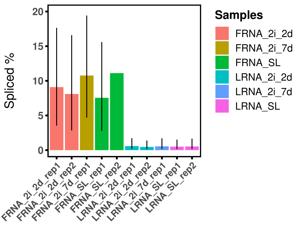
In this post, I will continue with reproducing the analysis from Shao et al and compare spliced reads across various 4sU labelled samples. The assumption is that in the short metabolic labelling experiments, the majority of reads should come from unspliced pre-mRNAs.
In order to extract spliced reads from the data, we will extract information in the 6th column of sam file (the CIGAR string) - see code below. The CIGAR string provides information on how your reads align to the reference sequence. Gaps in the alignments (indicative of splicing) are indicated as “N” in the CIGAR string. I refer you to the following blog for a really clear information on the CIGAR
samtools view -h alignment.bam | awk '$6 ~ /N/ || $1 ~ /^@/' | samtools view -bS - > spliced.bam
The first part of the statement uses samtools view to convert the bam to sam and include the header (-h). The awk command is then used to filter reads that contain N in the 6th column (the CIGAR string) or start with @ (therefore are header). The second view statement converts the output back to bam format.
To measure spliced reads in TT-seq I then followed Shao’s script with slight modifications:
setwd("your/working/dir")
source("dir/with/shaos/utils.R")
pacman::p_load(Rsubread, org.Mm.eg.db, TxDb.Mmusculus.UCSC.mm10.knownGene)

# get genes intervals
gene.gr <- GenomicFeatures::genes(TxDb.Mmusculus.UCSC.mm10.knownGene::TxDb.Mmusculus.UCSC.mm10.knownGene)
gene.gr <- gene.gr[!duplicated(ranges(gene.gr))]

ks <- keys(org.Mm.eg.db, keytype = "ENSEMBL")
res <- biomaRt::select(org.Mm.eg.db, keys = ks, keytype = "ENSEMBL",
                       columns = c("ENTREZID", "SYMBOL"))

gene.ann <- data.frame(GeneID = res$ENSEMBL[match(gene.gr$gene_id, res$ENTREZID)],
                       Chr = seqnames(gene.gr),
                       Start = start(gene.gr),
                       End = end(gene.gr),
                       Strand = strand(gene.gr))
gene.ann <- gene.ann[!is.na(gene.ann$GeneID), ]
Next, get sample sizes method. I used DESeq2
library(DESeq2)
#read in the file previously created for spike counts
spike_matrix_label=read.table(spike_matrix_label, file="spikematrix_L.txt", row.names=TRUE, col.names=TRUE)
samples_L<-c("LRNA_2i_2d_rep1","LRNA_2i_2d_rep2", "LRNA_2i_7d_rep1","LRNA_SL_rep1", "LRNA_SL_rep2")
cond_L<-c("2d","2d","7d","SL", "SL")
meta_L<-as.matrix(data.frame(samples_L,cond_L))
#here input from counts.rmd
dds_L<-DESeqDataSetFromMatrix(countData=spike_matrix_label,
                              colData=meta_L,
                              design= ~ cond_L)
dds_L <- estimateSizeFactors(dds_L)

LRNA.sizefactor<-sizeFactors(dds_L)
Count total and spliced reads
# count total reads
bam_files <- list.files("/your/working/dir/bams", pattern = ".bam$", full.names = T)
fc_PE <- Rsubread::featureCounts(bam_files, annot.ext=gene.ann, isPairedEnd=TRUE)

#size factor required here
#divide each count by appropriate size factor
readCounts<-fc_PE$counts
readCounts_scaled<-sweep(readCounts, 2, LRNA.sizefactor, '/')

# count spliced reads
spliced_bam_files <- list.files("/your/working/dir//spliced/", pattern = ".bam$", full.names = T)
fc_PE_spliced <- Rsubread::featureCounts(spliced_bam_files, annot.ext=gene.ann, isPairedEnd=TRUE)

#size factor required here
#divide each count by appropriate size factor
readCounts_spliced<-fc_PE_spliced$counts
readCounts_spliced_scaled<-sweep(readCounts_spliced, 2, LRNA.sizefactor, '/')

# get spliced ratio
spliced_ratio <- readCounts_spliced_scaled / readCounts_scaled
spliced_ratio <- spliced_ratio[rowSums(readCounts_scaled) > 0, ] # remove inactive genes
spliced_ratio <- spliced_ratio[!apply(spliced_ratio, 1, function(x) any(is.na(x) | is.infinite(x))), ]
# remove unspliced genes, counts true or false, so
#we have 6 types of samples, at least 6 x>0

spliced_ratio <- spliced_ratio[apply(spliced_ratio, 1, function(x) sum(x > 0) > 4), ] # remove unspliced genes
colnames(spliced_ratio)<-  c("FRNA_2i_2d_rep1", "FRNA_2i_2d_rep2", "FRNA_2i_7d_rep1", "FRNA_SL_rep1","FRNA_SL_rep2", "LRNA_2i_2d_rep1", "LRNA_2i_2d_rep2", "LRNA_2i_7d_rep1", "LRNA_SL_rep1","LRNA_SL_rep2")

### make the table for data - table with medians etc.
#create matrix
cellCountsmine=data.frame(

  # Taking sequence of elements
  c("FRNA_2i_2d_rep1", "FRNA_2i_2d_rep2", "FRNA_2i_7d_rep1", "FRNA_SL_rep1","FRNA_SL_rep2", "LRNA_2i_2d_rep1", "LRNA_2i_2d_rep2", "LRNA_2i_7d_rep1", "LRNA_SL_rep1","LRNA_SL_rep2"),

  # No of rows
  nrow = 10,

  # No of columns
  ncol = 1,

  # By default matrices are in column-wise order
  # So this parameter decides how to arrange the matrix
  byrow = TRUE
)

colnames(cellCountsmine) = c("Samples")
cellCountsmine$Spliced <- matrixStats::colMedians(spliced_ratio)[match(cellCountsmine$Samples, colnames(spliced_ratio))]
cellCountsmine$Spliced_lower <- apply(spliced_ratio, 2, function(x) quantile(x, 0.25))[match(cellCountsmine$Samples, colnames(spliced_ratio))]
cellCountsmine$Spliced_upper <- apply(spliced_ratio, 2, function(x) quantile(x, 0.75))[match(cellCountsmine$Samples, colnames(spliced_ratio))]
cellCountsmine$Spliced_sd <- colSds(spliced_ratio)[match(cellCountsmine$Samples, colnames(spliced_ratio))]
cellCountsmine$Spliced_mean <-  colMeans(spliced_ratio)[match(cellCountsmine$Samples, colnames(spliced_ratio))]
cellCountsmine$Color <- gsub("(.*)\\_rep.*", "\\1", cellCountsmine$Samples)

write.table(cellCountsmine, "/your/working/dir/Splicing_cell_number.txt",
            quote = F, row.names = F, col.names = T, sep = "\t")
Statistical tests and plotting
spliced_ratio2 <- spliced_ratio[, !grepl("2i_7d", colnames(spliced_ratio))]
spliced_ratio_mean <- sapply(c("2i_2d", "SL"),
                             function(x) rowMeans(spliced_ratio2[, grep(x, colnames(spliced_ratio2))])) %>%
  as.data.frame()
colMedians(as.matrix(spliced_ratio_mean))
colMeans(as.matrix(spliced_ratio_mean))

plot(density(log(spliced_ratio_mean$`2i_2d`/ spliced_ratio_mean$SL), na.rm = T))

median(na.omit((spliced_ratio_mean$`2i_2d` / spliced_ratio_mean$SL))) # 0.9686969

inf.omit = function(x) x[is.infinite(x)]
##Go through each row and determine if a value is zero
row_sub = apply(spliced_ratio_mean, 1, function(row) all(row !=0 ))
##Subset as usual
spliced_ratio_mean=spliced_ratio_mean[row_sub,]
t.test(na.omit( log2(spliced_ratio_mean$SL / spliced_ratio_mean$`2i_2d`))) # p-value < 2.2e-16

MASS::glm.nb(SL ~ `2i_2d`, data = spliced_ratio_mean) %>% summary()

# --------------------------------------------------------------------------------------------
cellCounts <- read.table("/your/working/dir/Splicing_cell_number.txt", header = T)
cellCounts$Samples <- factor(cellCounts$Samples, unique(cellCounts$Samples))

# plot
ggplot(cellCounts, aes(x = Samples, y = Spliced * 100, fill = Color)) +
  geom_bar(stat = "identity") +
  geom_linerange(aes(ymin=Spliced_lower * 100, ymax=Spliced_upper * 100)) +
  xlab("") +
  ylab("Spliced %\n") +
  ylim(0, 20) +
  labs(fill='Samples') +
  theme_setting +
  theme(axis.text.x = element_text(size = 11, angle = 45, hjust=1))

ggsave(filename = "splicing.pdf", path = "/your/working/dir/analysis/", device = "pdf",
       width = 5, height = 4)
The code results in the following plot:
 References:
1) Shao R, Kumar B, Lidschreiber K, Lidschreiber M, Cramer P, Elsässer SJ (2022). "Distinct transcription kinetics of pluripotent cell states."
Molecular Systems Biology (2022)18:e10407
2) Love MI, Huber W, Anders S (2014). “Moderated estimation of fold change and dispersion for RNA-seq data with DESeq2.” Genome Biology, 15, 550