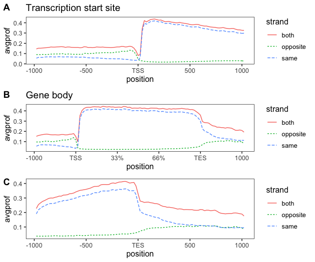
In this post, I will re-plot the graphs created using ngsplot, to combine the sense and anti-sense profiles on a single set of axes. Code from this blog was very useful as a starting point. All is done using R.
Load some essential packages:
library("dplyr")
library("ggplot2")
library("cowplot")
theme_set(theme_bw(base_size = 12))
theme_update(panel.grid.minor.x = element_blank(),
             panel.grid.minor.y = element_blank(),
             panel.grid.major.x = element_blank(),
             panel.grid.major.y = element_blank())
- Create functions, that aggregate results from different ngs runs.
- The purpose of this code is to create a big table with data for sense, both or anti-sense strands over TSS, TES and genebody. I used mostly code from this blog, but since part of their code was not functional (in my R session at least), I made the required updates.
import_ngsplot <- function(results, id = 1:length(results)) {
  # Imports and combines results from multiple ngsplot analyses
  #
  # results - name of ngsplot results (specified with -O flag)
  # id - description of analysis
  stopifnot(length(results) > 0, length(results) == length(id))
  avgprof_list <- list()
  sem_list <- list()
  for (i in seq_along(results)) {
    zipfile <- paste0(results[i], ".zip")
    extract_zip(zipfile)
    # Import mean coverage
    avgprof_list[[i]] <- import_data(path = results[i], datatype = "avgprof",
                                     id = id[i])
    # Import standard error of mean coverage
    sem_list[[i]] <- import_data(path = results[i], datatype = "sem",
                                id = id[i])
  }
  avgprof_df <- do.call(rbind, avgprof_list)
  colnames(avgprof_df)<-c("avgprof","position","id","metainfo")
  sem_df <- do.call(rbind, sem_list)
  colnames(sem_df)<-c("sem","position","id","metainfo")
  final <- merge(avgprof_df, sem_df,by=c("id","position"))
  return(final)
}

extract_zip <- function(zipfile) {
  # Unzip the ngsplot results into the same directory
  stopifnot(length(zipfile) == 1, file.exists(zipfile))
  unzip(zipfile, exdir = dirname(zipfile))
  return(invisible())
}

import_data <- function(path, datatype, id) {
  # Import the data from a specific ngsplot file.
  #
  # path - path to the ngsplot results directory
  # datatype - either "avgprof" for the mean coverage or
  #            "sem" for the standard error of the mean coverage
  # id - description of analysis (length == 1)
  stopifnot(datatype == "avgprof" | datatype == "sem",
            length(id) == 1)
  fname <- paste0(path, "/", datatype, ".txt")
  df <- read.delim(fname)
  df$position <- paste0("p", 1:nrow(df))
  df$id <- id
  df$metainfo<-id
  df$position <- sub("^p", "", df$position)
  df$position <- as.numeric(df$position)
  return(df)
}
- Import the data from specified location, using functions above:
cov <- import_ngsplot(results = c("/Users/mmaslon/Documents/jobs/poznan/analysis/TUannotation/bams/metaprofiles/LRNA_2i_7d_rep1.mate1.reheader.tss.both","/Users/mmaslon/Documents/jobs/poznan/analysis/TUannotation/bams/metaprofiles/LRNA_2i_7d_rep1.mate1.reheader.genebody.both","/Users/mmaslon/Documents/jobs/poznan/analysis/TUannotation/bams/metaprofiles/LRNA_2i_7d_rep1.mate1.reheader.tes.both","/Users/mmaslon/Documents/jobs/poznan/analysis/TUannotation/bams/metaprofiles/LRNA_2i_7d_rep1.mate1.reheader.tss.same","/Users/mmaslon/Documents/jobs/poznan/analysis/TUannotation/bams/metaprofiles/LRNA_2i_7d_rep1.mate1.reheader.genebody.same","/Users/mmaslon/Documents/jobs/poznan/analysis/TUannotation/bams/metaprofiles/LRNA_2i_7d_rep1.mate1.reheader.tes.same","/Users/mmaslon/Documents/jobs/poznan/analysis/TUannotation/bams/metaprofiles/LRNA_2i_7d_rep1.mate1.reheader.tss.opposite","/Users/mmaslon/Documents/jobs/poznan/analysis/TUannotation/bams/metaprofiles/LRNA_2i_7d_rep1.mate1.reheader.genebody.opposite","/Users/mmaslon/Documents/jobs/poznan/analysis/TUannotation/bams/metaprofiles/LRNA_2i_7d_rep1.mate1.reheader.tes.opposite"),id = c("tss-both", "genebody-both", "tes-both","tss-same", "genebody-same", "tes-same","tss-opposite","genebody-opposite","tes-opposite"))

#
cov <- separate(cov, "id", into = c("feature", "strand"), sep = "-")
cov$id <- factor(cov$feature, levels = c("tss", "genebody", "tes"))
- Draw plots (my own code, but code in the above mentioned blog works very nicely too).
p1<-ggplot(cov[cov$feature == "tss", ],aes(x=position,y=avgprof))+geom_line(aes(color = strand, linetype = strand)) + scale_x_continuous(breaks = c(0, 25, 50, 75, 100),
                     labels = c(-1000, -500, "TSS", 500, 1000)) +
  labs(title = "Transcription start site")

p2<-ggplot(cov[cov$feature == "tes", ],aes(x=position,y=avgprof))+geom_line(aes(color = strand, linetype = strand)) + scale_x_continuous(breaks = c(0, 25, 50, 75, 100),
                     labels = c(-1000, -500, "TES", 500, 1000))

p3<-ggplot(cov[cov$feature == "genebody", ],aes(x=position,y=avgprof))+geom_line(aes(color = strand, linetype = strand))+ scale_x_continuous(breaks = c(0, 20, 40, 60, 80, 100),
                     labels = c(-1000, "TSS", "33%", "66%", "TES", 1000)) +
  labs(title = "Gene body")

plot_grid(p1, p3, p2, nrow = 3, labels = LETTERS[1:3])
The above code results in the following image:
 ```{r}
sessionInfo()
R version 4.0.3 (2020-10-10)
Platform: x86_64-apple-darwin17.0 (64-bit)
Running under: macOS 12.5.1
Matrix products: default
LAPACK: /Library/Frameworks/R.framework/Versions/4.0/Resources/lib/libRlapack.dylib
Random number generation:
RNG: Mersenne-Twister
Normal: Inversion
Sample: Rounding
locale:
[1] en_US.UTF-8/en_US.UTF-8/en_US.UTF-8/C/en_US.UTF-8/en_US.UTF-8
attached base packages:
[1] stats graphics grDevices utils datasets methods base
other attached packages:
[1] cowplot_1.1.1 ggplot2_3.3.6 dplyr_1.0.8 tidyr_1.2.0
loaded via a namespace (and not attached):
[1] MatrixGenerics_1.2.1 Biobase_2.50.0 httr_1.4.3
[4] bit64_4.0.5 assertthat_0.2.1 askpass_1.1
[7] stats4_4.0.3 BiocFileCache_1.14.0 blob_1.2.3
[10] GenomeInfoDbData_1.2.4 Rsamtools_2.6.0 yaml_2.3.5
[13] progress_1.2.2 pillar_1.8.0 RSQLite_2.2.12
[16] lattice_0.20-45 glue_1.6.2 digest_0.6.29
[19] GenomicRanges_1.42.0 XVector_0.30.0 colorspace_2.0-3
[22] htmltools_0.5.2 Matrix_1.4-1 XML_3.99-0.9
[25] pkgconfig_2.0.3 biomaRt_2.46.3 zlibbioc_1.36.0
[28] purrr_0.3.4 scales_1.2.0 BiocParallel_1.24.1
[31] tibble_3.1.6 openssl_2.0.0 farver_2.1.0
[34] generics_0.1.3 IRanges_2.24.1 ellipsis_0.3.2
[37] withr_2.5.0 cachem_1.0.6 pacman_0.5.1
[40] SummarizedExperiment_1.20.0 GenomicFeatures_1.42.3 BiocGenerics_0.36.1
[43] cli_3.2.0 magrittr_2.0.3 crayon_1.5.1
[46] memoise_2.0.1 evaluate_0.15 fansi_1.0.3
[49] xml2_1.3.3 tools_4.0.3 prettyunits_1.1.1
[52] hms_1.1.1 lifecycle_1.0.1 matrixStats_0.61.0
[55] stringr_1.4.0 S4Vectors_0.28.1 munsell_0.5.0
[58] DelayedArray_0.16.3 AnnotationDbi_1.52.0 Biostrings_2.58.0
[61] compiler_4.0.3 GenomeInfoDb_1.26.7 rlang_1.0.2
[64] grid_4.0.3 RCurl_1.98-1.6 rstudioapi_0.13
[67] rappdirs_0.3.3 labeling_0.4.2 bitops_1.0-7
[70] rmarkdown_2.14 Rsubread_2.4.3 gtable_0.3.0
[73] DBI_1.1.3 curl_4.3.2 R6_2.5.1
[76] GenomicAlignments_1.26.0 knitr_1.39 rtracklayer_1.50.0
[79] fastmap_1.1.0 bit_4.0.4 utf8_1.2.2
[82] stringi_1.7.6 parallel_4.0.3 Rcpp_1.0.8.3
[85] vctrs_0.4.0 dbplyr_2.1.1 tidyselect_1.1.2
[88] xfun_0.30
```